Pruning Demo
In this demo we will show you how to:
Use the pruning functionality in
SymbolicModelto restrict output dimensions of a PyTorch MLPSet up a pruning schedule and train
Perform symbolic regression on a pruned MLP
Pruning Background
For interpretability purposes, it is good to reduce the dimensionality of deep learning models. High-dimensional representations often entangle multiple features, making it difficult to extract clear, human-understandable relationships. By encouraging a sparse representation, we encourage the network to compress information into a smaller set of meaningful components. This may also make symbolic regression possible on these models.
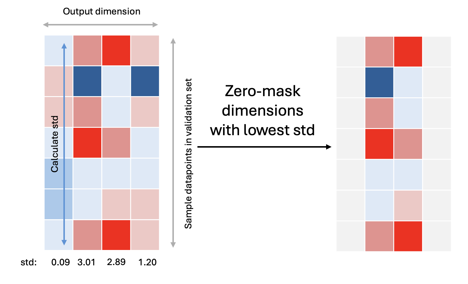
The SymTorch pruning class allows you to dynamically reduce the output dimensionality of MLPs by zero-masking the unimportant dimensions.
Important dimensions: The dimensions that the model uses the most in predicting the output. These would vary most with differences in the input. Hence we choose the important dimensions as the ones with the highest standard deviation across the datapoints.
We pass some input data through the model (usually a subset of the validation set) and analyse the outputs of the MLP. We choose the output dimensions that have the highest standard deviation across the datapoints, as shown below.
Wrapping a PyTorch model
Create a simple PyTorch model.
import torch
import numpy as np
import torch.nn as nn

class MLP(nn.Module):
    """
    Simple MLP.
    """
    def __init__(self, input_dim, output_dim, hidden_dim):
        super(MLP, self).__init__()
        self.mlp = nn.Sequential(
            nn.Linear(input_dim, hidden_dim),
            nn.ReLU(),
            nn.Dropout(0.2),
            nn.Linear(hidden_dim, hidden_dim),
            nn.ReLU(),
            nn.Dropout(0.2),
            nn.Linear(hidden_dim, hidden_dim),
            nn.ReLU(),
            nn.Dropout(0.2),
            nn.Linear(hidden_dim, output_dim)
        )

    def forward(self, x):
        return self.mlp(x)

class SimpleModel(nn.Module):
    """
    Model with MLP f_net and linear g_net.
    """
    def __init__(self, input_dim, output_dim, output_dim_f=32, hidden_dim=128):
        super(SimpleModel, self).__init__()

        self.f_net = MLP(input_dim, output_dim_f, hidden_dim)
        # g is linear - only learns to combine the 2 pruned outputs from f
        self.g_net = nn.Linear(output_dim_f, output_dim)  # Will use first 2 dims of f after pruning

    def forward(self, x):
        x = self.f_net(x)
        x = self.g_net(x)
        return x
Train the model on some data. We have a composite function \(y=g(f(\mathbf{x}))\).
and \(g\) is just a linear transformation of \(f_0\) and \(f_1\)
import numpy as np

# Make the dataset
x = np.array([np.random.uniform(0, 1, 10_000) for _ in range(5)]).T

def f_func(x):
    f0 = x[:, 0]**2
    f1 = np.sin(x[:, 4])
    return np.stack([f0, f1], axis=1)

def g_func(f_output):
    a, b = 2.5, -1.3
    return a * f_output[:, 0] + b * f_output[:, 1]

# Generate ground truth data
f_true = f_func(x)
y = g_func(f_true)

noise = np.array([np.random.normal(0, 0.05*np.std(y)) for _ in range(len(y))])
y = y + noise
We need to set up the pruning model.
from symtorch import SymbolicModel
Detected IPython. Loading juliacall extension. See https://juliapy.github.io/PythonCall.jl/stable/compat/#IPython
# Create model with pruning for f, linear g_net
model = SimpleModel(input_dim=x.shape[1], output_dim=1, output_dim_f=32)
model.f_net = SymbolicModel(model.f_net, block_name="f_net")

# Set up pruning
epochs = 100
batch_size = 32
steps_per_epoch = x.shape[0]/batch_size
total_steps = epochs * steps_per_epoch
model.f_net.setup_pruning(initial_dim=32,
                          target_dim=2, #dims at the end of pruning
                          end_step_frac=0.5, #when to finish pruning eg. ~50% of the way through training
                          decay_rate='exp',
                          total_steps=int(total_steps))
✅ Pruning successfully set up for block f_net.
   Initial dimensions: 32
   Target dimensions: 2
   Total steps: 31250
   Pruning will complete at step 15625
Training our model and dynamically reducing dimensionality
# Set up training

import torch.optim as optim
from torch.utils.data import DataLoader, TensorDataset
from sklearn.model_selection import train_test_split

def train_model(model, dataloader, X_val, opt, criterion, epochs=100):
    """
    Train model with MLP f (with pruning) and linear g_net.

    Args:
        model: PyTorch model to train
        dataloader: DataLoader for training data
        X_val, y_val: Validation data for pruning
        opt: Optimizer
        criterion: Loss function
        epochs: Number of training epochs

    Returns:
        tuple: (trained_model, loss_tracker, active_dims_tracker)
    """
    loss_tracker = []
    active_dims_tracker = []

    step = 0
    for epoch in range(epochs):
        epoch_loss = 0.0

        for batch_x, batch_y in dataloader:
            # Forward pass
            pred = model(batch_x)
            loss = criterion(pred, batch_y)
            # Backward pass
            opt.zero_grad()
            loss.backward()
            opt.step()

            epoch_loss += loss.item()

            model.f_net.prune(step, sample_data = X_val, # Pass in the validation set (or a subset of) to the model
                    parent_model = model) # Pass in the parent model to get the correct inputs to the layer

            step+=1

        loss_tracker.append(epoch_loss)
        active_dims_tracker.append(model.f_net.pruning_mask.sum().item())


        if (epoch + 1) % 10 == 0:
            avg_loss = epoch_loss / len(dataloader)
            active_dims = model.f_net.pruning_mask.sum().item()
            print(f'Epoch [{epoch+1}/{epochs}], Avg Loss: {avg_loss:.6f}, Active dims: {active_dims}')

    return model, loss_tracker, active_dims_tracker

# Set up training
criterion = nn.MSELoss()
opt = optim.Adam(model.parameters(), lr=0.001)
# Split data
X_train, X_val, y_train, y_val = train_test_split(
    x, y.reshape(-1,1), test_size=0.1, random_state=290402)

# Set up dataset - only x as input now
dataset = TensorDataset(torch.FloatTensor(X_train), torch.FloatTensor(y_train))
dataloader = DataLoader(dataset, batch_size=batch_size, shuffle=True)
# Train the model and save the weights
print("Starting training...")
model, losses, active_dims = train_model(model, dataloader, torch.FloatTensor(X_val), opt, criterion, 100)
print("Training completed!")
torch.save(model.state_dict(), 'model_weights.pth')
Starting training...
Epoch [10/100], Avg Loss: 0.002543, Active dims: 18
Epoch [20/100], Avg Loss: 0.002195, Active dims: 11
Epoch [30/100], Avg Loss: 0.002210, Active dims: 6
Epoch [40/100], Avg Loss: 0.002022, Active dims: 4
Epoch [50/100], Avg Loss: 0.001870, Active dims: 2
Epoch [60/100], Avg Loss: 0.001901, Active dims: 2
Epoch [70/100], Avg Loss: 0.001836, Active dims: 2
Epoch [80/100], Avg Loss: 0.001824, Active dims: 2
Epoch [90/100], Avg Loss: 0.001841, Active dims: 2
Epoch [100/100], Avg Loss: 0.001829, Active dims: 2
Training completed!
Let’s see how the number of active dimensions decrease as training progesses.
import matplotlib.pyplot as plt

plt.plot(active_dims)
plt.xlabel('Epochs')
plt.ylabel('Number of active dimensions for the f MLP output')
plt.show()

You can pass a decay_rate parameter into the .set_schedule method of a Pruning_MLP. The default is a cosine decay (as shown above). The other options are exp and linear.
 In the above image, the pruning finishes at epoch 75 and we prune 100 dimensions to 2 dimensions.
Interpret the MLP
The .distill function only takes into account the active (non-masked) dimensions.
print("\nRunning symbolic regression on pruned f...")

sr_params = {'complexity_of_operators':  {"sin":3, "exp":3},
             'complexity_of_constants': 2,
             'constraints': {"sin": 3, "exp":3},
             'parsimony': 0.01,
             'verbosity': 0,
             'niterations': 100}

model.f_net.distill(torch.FloatTensor(X_train),
                       sr_params=sr_params)
Running symbolic regression on pruned f...
🛠️ Running SR on active dimension 0 (1/2)
/Users/liz/PhD/SymTorch_project/symtorch_venv/lib/python3.11/site-packages/pysr/sr.py:2811: UserWarning: Note: it looks like you are running in Jupyter. The progress bar will be turned off.
  warnings.warn(
💡Best equation for active dimension 0: ((x0 * x0) * -9.177365) + (sin(x4) * (x0 + 3.7915835)).
🛠️ Running SR on active dimension 21 (2/2)
/Users/liz/PhD/SymTorch_project/symtorch_venv/lib/python3.11/site-packages/pysr/sr.py:2811: UserWarning: Note: it looks like you are running in Jupyter. The progress bar will be turned off.
  warnings.warn(
💡Best equation for active dimension 21: ((x0 * ((x4 * 0.02569695) + x0)) * 9.053295) + (sin(x4) * -4.9888153).
❤️ SR on f_net active dimensions complete.
{0: PySRRegressor.equations_ = [
 	    pick     score                                           equation  \
 	0         0.000000                                                 x4
 	1         0.222776                                         -1.0853426
 	2         0.308274                                     x0 * -3.806873
 	3         0.058161                               inv(x0 + -1.1267803)
 	4         0.431742                              x0 * (x0 * -5.707732)
 	5         0.477709                       (x0 * -8.686444) + 3.2480958
 	6         0.153751                      x4 + ((x0 * -6.5375166) * x0)
 	7         0.544373                (x0 * -7.4334426) + (x4 * 4.868192)
 	8         0.376226                ((x0 * x0) * -7.367284) + (x4 + x4)
 	9         3.306437         ((x0 * x0) * -8.744584) + (x4 * 3.6595654)
 	10        0.125803   (x4 * (x0 + 3.344076)) + (x0 * (x0 * -9.105152))
 	11        0.138711  ((x4 * 3.3089917) + ((x4 + -10.204634) * (x0 *...
 	12  >>>>  1.101763  ((x0 * x0) * -9.177365) + (sin(x4) * (x0 + 3.7...
 	13        0.090894  ((x0 * ((x0 * -1.7644632) + -0.17303404)) + si...
 	14        0.000671  (((((x0 + 0.09639773) * -1.7700083) * x0) + si...
 	15        0.074827  ((x0 + 4.5193567) * (sin(x4) + (x0 * (x0 * -1....
 	16        0.008228  ((sin(x4) + ((x0 * x0) * -1.5951045)) * (x0 + ...

 	        loss  complexity
 	0   9.869409           1
 	1   7.898432           2
 	2   4.263609           4
 	3   4.022708           5
 	4   2.612253           6
 	5   1.620126           7
 	6   1.389234           8
 	7   0.806041           9
 	8   0.553305          10
 	9   0.020277          11
 	10  0.015766          13
 	11  0.011947          15
 	12  0.003970          16
 	13  0.003022          19
 	14  0.003016          22
 	15  0.002799          23
 	16  0.002730          26
 ],
 21: PySRRegressor.equations_ = [
 	    pick     score                                           equation  \
 	0         0.000000                                                 x0
 	1         0.095859                                            x0 + x0
 	2         0.123548                                     x0 * 3.4731839
 	3         0.192502                              (x0 * x0) * 5.3865266
 	4         0.694850                     (x0 + -0.41388267) * 9.1824665
 	5         0.378998                (x0 * 7.6599708) + (x4 * -5.620235)
 	6         1.981346         (x0 * (x0 * 9.021318)) + (x4 * -4.3798647)
 	7         0.792054   (x4 * (x4 + -5.188016)) + ((x0 * 9.143758) * x0)
 	8         0.034904      (sin(x4) * -4.90822) + (x0 * (x0 * 9.136547))
 	9         0.003309  ((x0 * 9.15831) * x0) + (((x4 * 1.1163542) + -...
 	10        0.056247  ((sin(x4) * -4.863487) + -0.03387193) + ((x0 *...
 	11  >>>>  0.093207  ((x0 * ((x4 * 0.02569695) + x0)) * 9.053295) +...
 	12        0.015435  ((x0 + 0.0090198405) * (x0 * 8.947147)) + (sin...
 	13        0.063585  (sin(x4) * -5.000108) + ((((x4 + (x4 + x2)) * ...
 	14        0.001942  (((x0 * 9.004585) * x0) + (x2 * 0.044007648)) ...
 	15        0.022210  (sin(x4) * ((x0 * 0.31133893) + -5.0260777)) +...
 	16        0.000561  ((((x2 * 0.009918883) + (x0 + 0.0050150244)) *...

 	        loss  complexity
 	0   7.511932           1
 	1   6.201404           3
 	2   5.480674           4
 	3   3.729311           6
 	4   1.861484           7
 	5   0.872300           9
 	6   0.016584          11
 	7   0.003402          13
 	8   0.003285          14
 	9   0.003264          16
 	10  0.003085          17
 	11  0.002560          19
 	12  0.002445          22
 	13  0.002294          23
 	14  0.002281          26
 	15  0.002230          27
 	16  0.002227          30
 ]}
You can see that the outputs of the f_net NN are linear combinations of the f function.
model.f_net.show_symbolic_expression(dim=0)
➡️ Symbolic expressions for output dimension 0:
    complexity      loss                                           equation  \
0            1  9.869409                                                 x4
1            2  7.898432                                         -1.0853426
2            4  4.263609                                     x0 * -3.806873
3            5  4.022708                               inv(x0 + -1.1267803)
4            6  2.612253                              x0 * (x0 * -5.707732)
5            7  1.620126                       (x0 * -8.686444) + 3.2480958
6            8  1.389234                      x4 + ((x0 * -6.5375166) * x0)
7            9  0.806041                (x0 * -7.4334426) + (x4 * 4.868192)
8           10  0.553305                ((x0 * x0) * -7.367284) + (x4 + x4)
9           11  0.020277         ((x0 * x0) * -8.744584) + (x4 * 3.6595654)
10          13  0.015766   (x4 * (x0 + 3.344076)) + (x0 * (x0 * -9.105152))
11          15  0.011947  ((x4 * 3.3089917) + ((x4 + -10.204634) * (x0 *...
12          16  0.003970  ((x0 * x0) * -9.177365) + (sin(x4) * (x0 + 3.7...
13          19  0.003022  ((x0 * ((x0 * -1.7644632) + -0.17303404)) + si...
14          22  0.003016  (((((x0 + 0.09639773) * -1.7700083) * x0) + si...
15          23  0.002799  ((x0 + 4.5193567) * (sin(x4) + (x0 * (x0 * -1....
16          26  0.002730  ((sin(x4) + ((x0 * x0) * -1.5951045)) * (x0 + ...

       score                                       sympy_format  \
0   0.000000                                                 x4
1   0.222776                                  -1.08534260000000
2   0.308274                                     x0*(-3.806873)
3   0.058161                                 1/(x0 - 1.1267803)
4   0.431742                                  x0*x0*(-5.707732)
5   0.477709                         3.2480958 + x0*(-8.686444)
6   0.153751                            x0*(-6.5375166)*x0 + x4
7   0.544373                      x0*(-7.4334426) + x4*4.868192
8   0.376226                        x0*x0*(-7.367284) + x4 + x4
9   3.306437                   x0*x0*(-8.744584) + x4*3.6595654
10  0.125803             x0*x0*(-9.105152) + x4*(x0 + 3.344076)
11  0.138711         x0*x0*(x4 - 10.204634) + x0 + x4*3.3089917
12  1.101763       x0*x0*(-9.177365) + (x0 + 3.7915835)*sin(x4)
13  0.090894  (x0 + 3.811739)*(x0*(x0*(-1.7644632) - 0.17303...
14  0.000671  ((x0 + 0.09639773)*(-1.7700083)*x0 + sin(x4))*...
15  0.074827  (x0 + 4.5193567)*(x0*x0*(-1.5749025) + sin(x4)...
16  0.008228  (x0 + 4.476581)*(x0*x0*(-1.5951045) + sin(x4))...

                                        lambda_format
0                                 PySRFunction(X=>x4)
1                  PySRFunction(X=>-1.08534260000000)
2                     PySRFunction(X=>x0*(-3.806873))
3                 PySRFunction(X=>1/(x0 - 1.1267803))
4                  PySRFunction(X=>x0*x0*(-5.707732))
5         PySRFunction(X=>3.2480958 + x0*(-8.686444))
6            PySRFunction(X=>x0*(-6.5375166)*x0 + x4)
7      PySRFunction(X=>x0*(-7.4334426) + x4*4.868192)
8        PySRFunction(X=>x0*x0*(-7.367284) + x4 + x4)
9   PySRFunction(X=>x0*x0*(-8.744584) + x4*3.6595654)
10  PySRFunction(X=>x0*x0*(-9.105152) + x4*(x0 + 3...
11  PySRFunction(X=>x0*x0*(x4 - 10.204634) + x0 + ...
12  PySRFunction(X=>x0*x0*(-9.177365) + (x0 + 3.79...
13  PySRFunction(X=>(x0 + 3.811739)*(x0*(x0*(-1.76...
14  PySRFunction(X=>((x0 + 0.09639773)*(-1.7700083...
15  PySRFunction(X=>(x0 + 4.5193567)*(x0*x0*(-1.57...
16  PySRFunction(X=>(x0 + 4.476581)*(x0*x0*(-1.595...
🏆 Best: ((x0 * x0) * -9.177365) + (sin(x4) * (x0 + 3.7915835)) (loss: 3.969665e-03)
We can even perform SR on the g_net to show that this layer is just a linear transformation of the inputs.
Because g_net is an intermediate layer of the MLP, we need to pass in the parent_model (the whole model) to get the correct inputs to g_net for symbolic regression.
model.g_net = SymbolicModel(model.g_net, block_name='g_net')
model.g_net.distill(torch.FloatTensor(X_train),
                     parent_model=model, # Pass in the parent_model because g_net is an intermediate layer
                     sr_params = sr_params)
🛠️ Running SR on output dimension 0 of 0
/Users/liz/PhD/SymTorch_project/symtorch_venv/lib/python3.11/site-packages/pysr/sr.py:2811: UserWarning: Note: it looks like you are running in Jupyter. The progress bar will be turned off.
  warnings.warn(
💡Best equation for output 0 found to be (((x0 + 0.00012825789) * -0.104232065) + -0.0026094334) + (x21 * 0.17798738).
❤️ SR on g_net complete.
{0: PySRRegressor.equations_ = [
 	   pick         score                                           equation  \
 	0        0.000000e+00                                                x31
 	1        8.785424e-02                                         0.24939868
 	2        3.121439e+00                                    x21 * 0.2789512
 	3        5.638493e-01                    (x21 * 0.27616408) + 0.03388125
 	4        2.722068e+00           (x0 * -0.097962625) + (x21 * 0.18385741)
 	5        3.338238e-07     (x0 * -0.09796284) + ((x12 + 0.1838572) * x21)
 	6        1.949614e+01  ((x21 * 0.17798749) + (x0 * -0.10423195)) + -0...
 	7        2.760529e-01  (x21 * 0.17798734) + ((x26 + (x0 * -0.10423212...
 	8  >>>>  4.623406e-01  (((x0 + 0.00012825789) * -0.104232065) + -0.00...

 	           loss  complexity
 	0  7.395062e-01           1
 	1  6.773096e-01           2
 	2  1.316859e-03           4
 	3  2.426105e-04           7
 	4  1.048458e-06           9
 	5  1.048457e-06          11
 	6  3.576713e-15          12
 	7  2.059243e-15          14
 	8  1.296927e-15          15
 ]}
The variables used in this NN are just the active dimensions of the f_net NN.
Switch to Using the Equation Instead in the Forwards Pass
model.f_net.switch_to_symbolic()
✅ Successfully switched f_net to symbolic equations for 2 active dimensions:
   Dimension 0: ((x0 * x0) * -9.177365) + (sin(x4) * (x0 + 3.7915835))
   Variables: ['x0', 'x4']
   Dimension 21: ((x0 * ((x4 * 0.02569695) + x0)) * 9.053295) + (sin(x4) * -4.9888153)
   Variables: ['x0', 'x4']
🎯 Active dimensions [0, 21] now using symbolic equations.
🔒 Inactive dimensions will output zeros.
model.g_net.switch_to_symbolic()
✅ Successfully switched g_net to symbolic equations for all 1 dimensions:
   Dimension 0: (((x0 + 0.00012825789) * -0.104232065) + -0.0026094334) + (x21 * 0.17798738)
   Variables: ['x0', 'x21']
🎯 All 1 output dimensions now using symbolic equations.
Now when running the forwards pass through the model, it uses the symbolic equation instead of the MLP.
interpretable_outputs = model(torch.tensor(X_train, dtype=torch.float32))
interpretable_outputs
tensor([[-0.0244],
        [ 0.1939],
        [-0.4942],
        ...,
        [-0.7961],
        [ 1.8698],
        [ 1.2709]])
Switch to Using the MLP in the Forwards Pass
model.f_net.switch_to_block()
model.g_net.switch_to_block()
✅ Switched f_net back to block
✅ Switched g_net back to block
model.eval()
with torch.no_grad():
    model_outputs = model(torch.tensor(X_train, dtype=torch.float32))
model_outputs
tensor([[-0.0293],
        [ 0.1937],
        [-0.4943],
        ...,
        [-0.7949],
        [ 1.8919],
        [ 1.2544]])
# Clean up
import os
import shutil
if os.path.exists('SR_output'):
    shutil.rmtree('SR_output')
os.remove('model_weights.pth')