Physics-Informed Neural Network (PINN)

PINNs are is a NNs trained on data and a loss that penalises violations of the governing differential equations and boundary/initial conditions, so its predictions obey the underlying physics.
They can be useful in predicting behviour of physical systems, provided that obey known DEs, if we have a small amount of data.

In this demo, we show how SymTorch can be used to discover the true analytical solutions to three different PDEs,

1. Heat Equation

2. Wave Equation

3. Damped Harmonic Oscillator,

including the value of unknown constants!

Let’s start with trying to find the general solution of the 1D heat equation:

\[ \frac{\partial u}{\partial t} = \alpha \frac{\partial^2 u}{\partial x^2} \]

where \(u\) is the temperature, \(t\) is time, \(x\) is the 1D spatial coordinate and \(\alpha\) is a constant that determines how quickly the heat conducts through the material.

The initial condition (IC) is \(u(x,0)=\sin(\pi x)\) and the boundary conditions (BCs) are \(u(0,t)=u(1,t)=0\).

Let’s train a NN and a PINN on only 10 data points.

import torch
import torch.nn as nn
import numpy as np
np.random.seed(290402)

alpha = 0.2 # Set alpha

# Heat equation
def temp(x,t):
    return np.exp(-np.pi**2 * alpha * t) * np.sin(np.pi * x)

# Create 10 random points
N = 10
x = np.random.rand(N)
t = np.random.rand(N)

# Make the data points for training
xt = torch.tensor(np.stack([x, t], axis=1), dtype=torch.float32) 
u = torch.tensor(temp(x,t).reshape(-1,1), dtype=torch.float32)

# Create a regular NN

class RegularNN(nn.Module):
    def __init__(self, in_dim=2, out_dim=1, hidden_dim=32):
        super(RegularNN, self).__init__()
        self.net = nn.Sequential(
            nn.Linear(in_dim, hidden_dim),
            nn.Tanh(),
            nn.Linear(hidden_dim, hidden_dim),
            nn.Tanh(),
            nn.Linear(hidden_dim, hidden_dim),
            nn.Tanh(),
            nn.Linear(hidden_dim, out_dim)
        )
    
    def forward(self, x):
        return self.net(x)
    
    def predict(self, x):
        self.eval()
        return self.net(x)

The PINN has the same architecture as the previous NN but we can use PyTorch’s autodifferentiation to find \(u_{xx}\) and \(u_t\) and add regularisation terms to the loss:

\[ \mathcal{L}_{\mathrm{PDE}} = \lambda_{\mathrm{pde}}\,\frac{1}{N}\sum_{i=1}^{N} \left( u_t(x_i,t_i) - \alpha\,u_{xx}(x_i,t_i) \right)^2 \]

\[ \mathcal{L}_{\mathrm{BC}} = \lambda_{\mathrm{BC}}\,\frac{1}{N}\sum_{i=1}^{N} \left( u(0,t_i)^2 + u(1,t_i)^2 \right) \]

\[ \mathcal{L}_{\mathrm{IC}} = \lambda_{\mathrm{IC}}\,\frac{1}{N}\sum_{i=1}^{N} \left( u(x_i,0) - \sin(\pi x_i) \right)^2 \]

Another advantage of using a PINN is that we can set constants of the PDE (in this case \(\alpha\)) to be differentiable constants and we can extract their values from the trained PINN.

class PINN(RegularNN):
    def __init__(self, in_dim=2, out_dim=1, hidden_dim=32):
        super().__init__(in_dim=in_dim, out_dim=out_dim, hidden_dim=hidden_dim)

        self.type = 'pinn'
        self.alpha = nn.Parameter(data=torch.tensor([0.])) # Differentiable constant

    def pde_residual(self, xt):

        xt = xt.requires_grad_(True)              
        u  = self.forward(xt)                   

        grads = torch.autograd.grad(
            u, xt, torch.ones_like(u), create_graph=True
        )[0]                                     
        u_x = grads[:, 0:1]
        u_t = grads[:, 1:2]

        u_xx = torch.autograd.grad(
            u_x, xt, torch.ones_like(u_x), create_graph=True
        )[0][:, 0:1]

        res = u_t - self.alpha * u_xx
        return res
    
    def bc_residual(self, xt):
            t  = xt[:, 1:2].detach()                    
            x0 = torch.zeros_like(t)
            x1 = torch.ones_like(t)

            u0 = self.forward(torch.cat([x0, t], dim=1))  
            u1 = self.forward(torch.cat([x1, t], dim=1))  

            return torch.cat([u0, u1], dim=0)           

    def ic_residual(self, xt):

        x  = xt[:, 0:1].detach()                   
        t0 = torch.zeros_like(x)

        u_init = self.forward(torch.cat([x, t0], dim=1))
        target = torch.sin(torch.pi * x)

        return u_init - target                   

Let’s train the models.

import torch.optim as optim

def train(model, xt, u, epochs=3000, lr=1e-3, weight_decay=0.0, device="mps", verbose=False,
          reg_pde=1, reg_ic=5, reg_bc=5):

    model = model.to(device)
    xt = xt.to(device)
    u = u.to(device)

    model.train()
    opt = optim.Adam(model.parameters(), lr=lr, weight_decay=weight_decay)
    loss_fn = nn.MSELoss()

    loss_hist = []
    for ep in range(1, epochs+1):
        opt.zero_grad()
        pred = model(xt)
        loss = loss_fn(pred, u)

        if model.type == 'pinn':
            pde_res = model.pde_residual(xt)
            bc_res = model.bc_residual(xt)
            ic_res = model.ic_residual(xt)
            loss += reg_pde * (pde_res**2).mean() + reg_ic * (ic_res**2).mean() + reg_bc * (bc_res**2).mean()

        loss.backward()
        opt.step()
        loss_hist.append(loss.item())
        if verbose and ep % 500 == 0:
            print(f"[sup10] ep={ep} loss={loss.item():.3e}")

    return model, loss_hist

#Train the regular NN
regular_NN = RegularNN()
regular_NN, _ = train(regular_NN, xt, u)

# Save the mode weights|
torch.save(regular_NN.state_dict(), 'regular_NN.pth')

# Train the PINN
pinn = PINN()
pinn, _ = train(pinn, xt, u)

# Save the mode weights
torch.save(pinn.state_dict(), 'pinn.pth')

Let’s plot the predicted data from the regular NN and the PINN and compare them with the true form.

import matplotlib.pyplot as plt
plt.rcParams.update({
    "font.size": 18,
    "axes.titlesize": 18,
    "axes.labelsize": 18,
    "xtick.labelsize": 18,
    "ytick.labelsize": 18,
    "legend.fontsize": 18,
})

def make_2d_hists(nn_model, pinn_model, alpha=1.0, Nx=100, Nt=100):
    # space–time grid
    x = np.linspace(0.0, 1.0, Nx)
    t = np.linspace(0.0, 1.0, Nt)
    X, T = np.meshgrid(x, t, indexing="ij")  # X: (Nx,Nt), T: (Nx,Nt)

    # True solution
    U_exact = np.exp(-np.pi**2 * alpha * T) * np.sin(np.pi * X)

    def predict_grid(model):
        model.eval()
        device = next(model.parameters()).device
        XT = np.stack([X.ravel(), T.ravel()], axis=1)  # (Nx*Nt, 2) with [x,t]
        xt = torch.tensor(XT, dtype=torch.float32, device=device)
        with torch.no_grad():
            U = model(xt).reshape(Nx, Nt).detach().cpu().numpy()
        return U

    U_nn   = predict_grid(nn_model)
    U_pinn = predict_grid(pinn_model)

    vmin = min(U_exact.min(), U_nn.min(), U_pinn.min())
    vmax = max(U_exact.max(), U_nn.max(), U_pinn.max())

    fig, axes = plt.subplots(1, 3, figsize=(12, 4), constrained_layout = True)
    data_plots = [("True", U_exact), ("Regular NN", U_nn), ("PINN", U_pinn)]

    for ax, (title, U) in zip(axes, data_plots):
        im = ax.imshow(
            U,
            origin="lower",
            extent=[0, 1, 0, 1],
            aspect="auto",
            cmap="Blues",
            vmin=vmin,
            vmax=vmax
        )
        ax.set_xlabel("t")
        ax.set_ylabel("x")
        ax.set_title(title)

    # single shared colorbar
    cbar = fig.colorbar(
        im,
        ax=axes,
        location="right",
        fraction=0.025,
        pad=0.02,
    )
    cbar.set_label(r"$u(x,t)$")

    plt.savefig("pinn.png", dpi = 300)
    plt.show()

make_2d_hists(regular_NN, pinn, alpha=alpha)

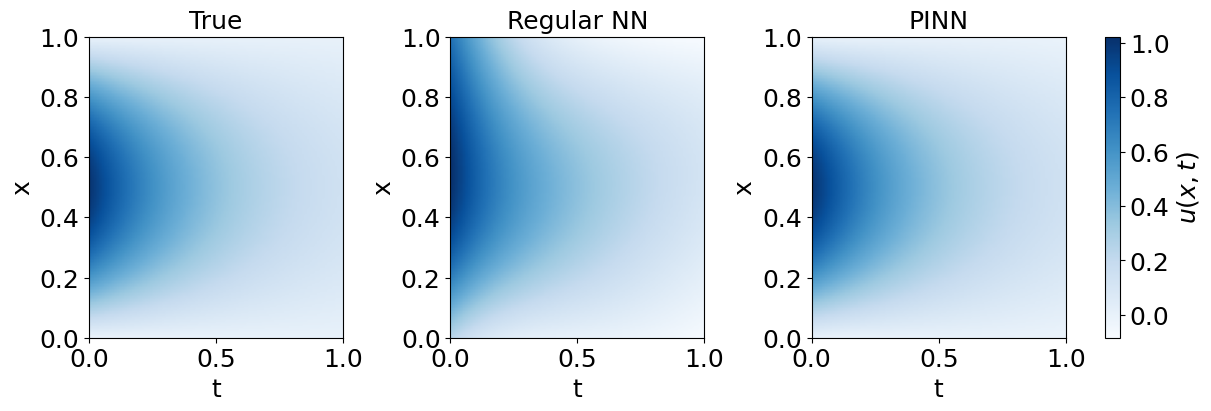
The PINN was much better at predicting the true temperatures than the regular NN with the same architecture.

Let’s see what the PINN predicts \(\alpha\) to be:

print(f"predicted alpha = {float(pinn.alpha):.3f}")

predicted alpha = 0.196

This is a pretty good estimate from the true \(\alpha=0.2\)

Now let’s see if we are able to distill the solution to the 1-D heat equation from the PINN.

Use PyTorch to approximate the behaviour of the PINN

from symtorch import SymbolicModel

num_data = 5000 # Create 5000 different data points
sample_data = torch.tensor(np.random.rand(num_data, 2), dtype=torch.float32) 
pinn.net = SymbolicModel(pinn.net, 'pinn')

sr_params = {'niterations': 1000,
             'constraints': {'sin':3, 'exp':3}, 
             'complexity_of_operators': {'sin':3, 'exp':3},
             "unary_operators": ["inv(x) = 1/x", "sin", "exp"],
             'parsimony': 0.01,
             'nested_constraints':{'sin':{'sin':0, 'exp':0}, 'exp':{'exp':0, 'sin':0}},
             'verbosity': 0
             }

variable_names = ['x', 't']
fit_params = {'variable_names': variable_names}

pinn.net.distill(sample_data.to(torch.device('mps')), sr_params = sr_params,
                 fit_params=fit_params
                 )

pinn.net.show_symbolic_expression(complexity=[13])

➡️ Dimension 0 - Complexity 13:
   sin(x * 3.1444418) * exp(t * -1.980765) (loss: 3.046010e-05)

The correct equation is of the form

\[ u(x,t) = e^{-\pi^2 \alpha t} \sin(\pi x) \approx e^{-1.97} \sin (3.14 x) \]

PySR’s best equation returns correct form of the equation!
(For more reliable SR performance, you should increase niterations until the Pareto front stablises, which may be >1000).

pinn.net.switch_to_symbolic(complexity=13)

✅ Successfully switched pinn to symbolic equations for all 1 dimensions:
   Dimension 0: sin(x * 3.1444418) * exp(t * -1.980765)
   Variables: ['t', 'x']
🎯 All 1 output dimensions now using symbolic equations.

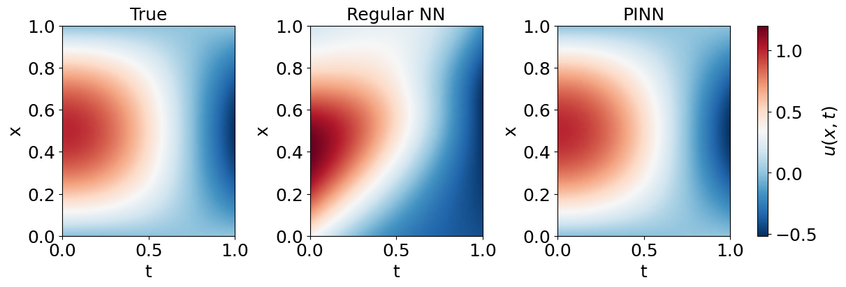
1D Wave Equation

The 1D wave equation:

\[ \frac{\partial^2 u}{\partial t^2} = c^2 \frac{\partial^2 u}{\partial x^2} \]

with IC \(u(x,0) = \sin(\pi x)\), \(\frac{\partial u}{\partial t}(x,0) = 0\) and BCs \(u(0,t) = u(1,t) = 0\).

The exact solution is \(u(x,t) = \sin(\pi x) \cos(c \pi t)\), and \(c\) is a learnable parameter.

c_true = 0.67

def wave_exact(x, t):
    return np.sin(np.pi * x) * np.cos(c_true * np.pi * t)

N = 10
x_wave = np.random.rand(N)
t_wave = np.random.rand(N)
xt_wave = torch.tensor(np.stack([x_wave, t_wave], axis=1), dtype=torch.float32)
u_wave = torch.tensor(wave_exact(x_wave, t_wave).reshape(-1, 1), dtype=torch.float32)

class WavePINN(RegularNN):
    def __init__(self, in_dim=2, out_dim=1, hidden_dim=32):
        super().__init__(in_dim=in_dim, out_dim=out_dim, hidden_dim=hidden_dim)
        self.type = 'pinn'
        self.c = nn.Parameter(data=torch.tensor([0.5]))

    def pde_residual(self, xt):
        xt = xt.requires_grad_(True)
        u = self.forward(xt)
        grads = torch.autograd.grad(u, xt, torch.ones_like(u), create_graph=True)[0]
        u_x = grads[:, 0:1]
        u_t = grads[:, 1:2]
        u_xx = torch.autograd.grad(u_x, xt, torch.ones_like(u_x), create_graph=True)[0][:, 0:1]
        u_tt = torch.autograd.grad(u_t, xt, torch.ones_like(u_t), create_graph=True)[0][:, 1:2]
        return u_tt - self.c**2 * u_xx

    def bc_residual(self, xt):
        t = xt[:, 1:2].detach()
        x0 = torch.zeros_like(t)
        x1 = torch.ones_like(t)
        u0 = self.forward(torch.cat([x0, t], dim=1))
        u1 = self.forward(torch.cat([x1, t], dim=1))
        return torch.cat([u0, u1], dim=0)

    def ic_residual(self, xt):
        x = xt[:, 0:1].detach()
        t0 = torch.zeros_like(x)
        xt0 = torch.cat([x, t0], dim=1).requires_grad_(True)
        u0 = self.forward(xt0)
        target = torch.sin(torch.pi * x)
        pos_residual = u0 - target
        grads = torch.autograd.grad(u0, xt0, torch.ones_like(u0), create_graph=True)[0]
        vel_residual = grads[:, 1:2]
        return torch.cat([pos_residual, vel_residual], dim=0)

wave_nn = RegularNN()
wave_nn, _ = train(wave_nn, xt_wave, u_wave, epochs=5000)

wave_pinn = WavePINN()
wave_pinn, _ = train(wave_pinn, xt_wave, u_wave, epochs=5000)

def plot_wave(nn_model, pinn_model, c=0.67, Nx=100, Nt=100):
    x = np.linspace(0.0, 1.0, Nx)
    t = np.linspace(0.0, 1.0, Nt)
    X, T = np.meshgrid(x, t, indexing="ij")

    U_exact = np.sin(np.pi * X) * np.cos(c * np.pi * T)

    def predict_grid(model):
        model.eval()
        device = next(model.parameters()).device
        XT = np.stack([X.ravel(), T.ravel()], axis=1)
        xt = torch.tensor(XT, dtype=torch.float32, device=device)
        with torch.no_grad():
            return model(xt).reshape(Nx, Nt).detach().cpu().numpy()

    U_nn = predict_grid(nn_model)
    U_pinn = predict_grid(pinn_model)

    vmin = min(U_exact.min(), U_nn.min(), U_pinn.min())
    vmax = max(U_exact.max(), U_nn.max(), U_pinn.max())

    fig, axes = plt.subplots(1, 3, figsize=(12, 4), constrained_layout=True)
    for ax, (title, U) in zip(axes, [("True", U_exact), ("Regular NN", U_nn), ("PINN", U_pinn)]):
        im = ax.imshow(U, origin="lower", extent=[0, 1, 0, 1], aspect="auto", cmap="RdBu_r", vmin=vmin, vmax=vmax)
        ax.set_xlabel("t")
        ax.set_ylabel("x")
        ax.set_title(title)

    fig.colorbar(im, ax=axes, location="right", fraction=0.025, pad=0.02).set_label(r"$u(x,t)$")
    plt.savefig("wave_pinn.png", dpi=300)
    plt.show()

plot_wave(wave_nn, wave_pinn, c=c_true)

print(f"predicted c = {float(wave_pinn.c):.3f}")

predicted c = 0.666

Distill the wave equation PINN with SymTorch

wave_pinn.net = SymbolicModel(wave_pinn.net, 'wave_pinn')

num_data = 5000
sample_data_wave = torch.tensor(np.random.rand(num_data, 2), dtype=torch.float32)

sr_params_wave = {
    'niterations': 1000,
    'constraints': {'sin': 3, 'cos': 3, 'exp': 3},
    'complexity_of_operators': {'sin': 3, 'cos': 3, 'exp': 3},
    'unary_operators': ['inv(x) = 1/x', 'sin', 'cos', 'exp'],
    'parsimony': 0.01,
    'nested_constraints': {
        'sin': {'sin': 0, 'cos': 0, 'exp': 0},
        'cos': {'cos': 0, 'sin': 0, 'exp': 0},
        'exp': {'exp': 0, 'sin': 0, 'cos': 0}
    },
    'verbosity': 0
}

variable_names = ['x', 't']
fit_params = {'variable_names': variable_names}

wave_pinn.net.distill(sample_data_wave.to(torch.device('mps')), sr_params=sr_params_wave, fit_params=fit_params)

wave_pinn.net.show_symbolic_expression(complexity=[13])

➡️ Dimension 0 - Complexity 13:
   sin(x * 3.1465797) * cos(t * 2.104846) (loss: 3.854858e-05)

The correct equation is of the form

\[ u(x,t) = \sin(\pi x) \cos(c \pi t) \approx \sin(3.14\, x) \cos(2.10\, t) \]

Damped Harmonic Oscillator

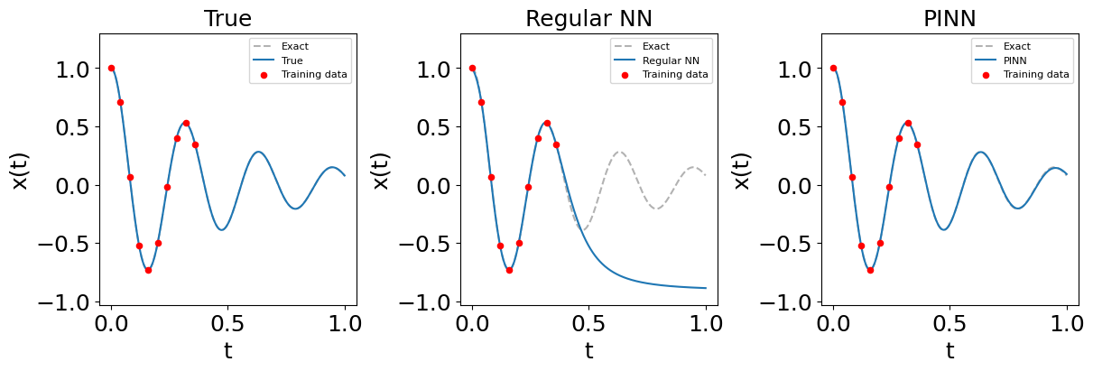
The damped harmonic oscillator ODE:

\[ \frac{d^2 x}{d t^2} + \mu \frac{d x}{d t} + k\, x = 0 \]

with ICs \(x(0) = 1\) and \(x'(0) = 0\).

We parameterise with \(\delta = \mu / 2\) and \(\omega_0 = \sqrt{k}\) (assuming unit mass). For the under-damped case (\(\delta < \omega_0\)), the exact solution is:

\[x(t) = e^{-\delta t}\left[2A\cos(\phi + \omega t)\right], \quad \omega = \sqrt{\omega_0^2 - \delta^2}, \quad \phi = \arctan\!\left(\frac{-\delta}{\omega}\right), \quad A = \frac{1}{2\cos\phi}\]

We use \(\delta = 2\), \(\omega_0 = 20\) on the domain \(t \in [0, 1]\).

This setup follows Moseley et al..

d, w0 = 2, 20  # delta (damping) and natural frequency
mu, k = 2*d, w0**2

# Exact analytical solution
w = np.sqrt(w0**2 - d**2)
phi = np.arctan(-d / w)
A = 1 / (2 * np.cos(phi))

def oscillator_exact(t):
    return np.exp(-d * t) * 2 * A * np.cos(phi + w * t)

# 500 evenly spaced points for evaluation
t_eval = np.linspace(0, 1, 500)
x_eval = oscillator_exact(t_eval)

# Training data: 10 points from the left portion of the domain
t_train = t_eval[0:200:20]  # indices 0, 20, 40, ..., 180 → ~10 points in [0, 0.4]
x_train = oscillator_exact(t_train)

t_train_tensor = torch.tensor(t_train.reshape(-1, 1), dtype=torch.float32)
x_train_tensor = torch.tensor(x_train.reshape(-1, 1), dtype=torch.float32)

print(f"Training points: {len(t_train)}, domain: [{t_train.min():.3f}, {t_train.max():.3f}]")

Training points: 10, domain: [0.000, 0.361]

class OscillatorNN(nn.Module):
    """Fully-connected network: 1 input → N_HIDDEN x N_LAYERS → 1 output, with Tanh activations."""
    def __init__(self, n_hidden=32, n_layers=3):
        super().__init__()
        activation = nn.Tanh
        self.fcs = nn.Sequential(nn.Linear(1, n_hidden), activation())
        self.fch = nn.Sequential(*[
            nn.Sequential(nn.Linear(n_hidden, n_hidden), activation()) for _ in range(n_layers - 1)
        ])
        self.fce = nn.Linear(n_hidden, 1)

    def forward(self, x):
        x = self.fcs(x)
        x = self.fch(x)
        x = self.fce(x)
        return x

class OscillatorPINN(OscillatorNN):
    def __init__(self, n_hidden=32, n_layers=3):
        super().__init__(n_hidden=n_hidden, n_layers=n_layers)
        self.type = 'pinn'

    def pde_residual(self, t_ignored):
        """Physics residual evaluated on a fixed grid of 30 collocation points."""
        t_physics = torch.linspace(0, 1, 30).view(-1, 1).to(next(self.parameters()).device).requires_grad_(True)
        x = self.forward(t_physics)
        dx = torch.autograd.grad(x, t_physics, torch.ones_like(x), create_graph=True)[0]
        dx2 = torch.autograd.grad(dx, t_physics, torch.ones_like(dx), create_graph=True)[0]
        residual = dx2 + mu * dx + k * x
        return residual

    # BCs don't apply in this PDE 
    def bc_residual(self, t):
        return torch.zeros(1, device=t.device)
    # ICs implicitly satisfied with the training data so ignore 
    def ic_residual(self, t):
        return torch.zeros(1, device=t.device)

torch.manual_seed(290402)

# Train regular NN
osc_nn = OscillatorNN()
osc_nn, _ = train(osc_nn, t_train_tensor, x_train_tensor, epochs=20000, lr=1e-3)

# Train PINN
osc_pinn = OscillatorPINN()
osc_pinn, _ = train(osc_pinn, t_train_tensor, x_train_tensor, epochs=20000, lr=1e-4,
                    reg_pde=1e-4, reg_ic=0, reg_bc=0)

def plot_oscillator(nn_model, pinn_model):
    t = np.linspace(0, 1, 500)
    x_true = oscillator_exact(t)

    def predict(model):
        model.eval()
        device = next(model.parameters()).device
        t_tensor = torch.tensor(t.reshape(-1, 1), dtype=torch.float32, device=device)
        with torch.no_grad():
            return model(t_tensor).cpu().numpy().flatten()

    x_nn = predict(nn_model)
    x_pinn = predict(pinn_model)

    fig, axes = plt.subplots(1, 3, figsize=(12, 4), constrained_layout=True)
    for ax, (title, x_pred) in zip(axes, [("True", x_true), ("Regular NN", x_nn), ("PINN", x_pinn)]):
        ax.plot(t, x_true, 'k--', alpha=0.3, label="Exact")
        ax.plot(t, x_pred, label=title)
        ax.scatter(t_train, x_train, c='red', s=20, zorder=5, label="Training data")
        ax.set_xlabel("t")
        ax.set_ylabel("x(t)")
        ax.set_title(title)
        ax.set_ylim(x_true.min() - 0.3, x_true.max() + 0.3)
        ax.legend(fontsize=8)

    plt.savefig("oscillator_pinn.png", dpi=300)
    plt.show()

plot_oscillator(osc_nn, osc_pinn)

Distill the oscillator PINN with SymTorch

osc_symbolic = SymbolicModel(osc_pinn, 'oscillator_pinn')

num_data = 5000
sample_data_osc = torch.tensor(np.random.uniform(0, 1, (num_data, 1)), dtype=torch.float32)

sr_params_osc = {
    'niterations': 1000,
    'constraints': {'sin': 3, 'cos': 3, 'exp': 3},
    'complexity_of_operators': {'sin': 3, 'cos': 3, 'exp': 3},
    'unary_operators': ['inv(x) = 1/x', 'sin', 'cos', 'exp'],
    'parsimony': 0.01,
    'nested_constraints': {
        'sin': {'sin': 0, 'cos': 0, 'exp': 0},
        'cos': {'cos': 0, 'sin': 0, 'exp': 0},
        'exp': {'exp': 0, 'sin': 0, 'cos': 0}
    },
    'verbosity': 0
}

fit_params = {'variable_names': ['t']}

osc_symbolic.distill(sample_data_osc.to(torch.device('mps')), sr_params=sr_params_osc, fit_params=fit_params)

osc_symbolic.show_symbolic_expression(complexity=[13])

➡️ Dimension 0 - Complexity 13:
   exp(t * -1.9995654) * cos(t * -19.624798) (loss: 5.038163e-04)

The exact solution is:

\[ x(t) = e^{-2t}\left[2A\cos(\phi + \sqrt{396}\, t)\right] \]

where \(\omega = \sqrt{20^2 - 2^2} = \sqrt{396} \approx 19.9\), \(2A \approx 1\) and \(\phi \approx -0.1\). The symbolic distillation may be able to recover \(\phi\) with more iterations, but struggles due to its small magnitude!